1 Overview

This assignment may result in several different programs. Instead of make run we will use several different make targets, one for each broad simulation type.

The required part of this assignment is earn 50 points on this assignment. The optional part is any points in excess of 50 that you earn.

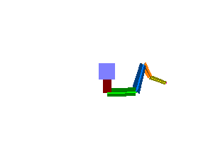
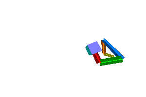
1.1 make bones file=filename (15–100 points)

This is an extension of HW4: everything that was required in HW4 is required in this program too.

You may find our bones writeup and change of basis writeup to be helpful.

bone d

This may appear at most once in any object. If present, it means that this object is considered to be a bone, with object-space origin (0,0,0) and object-space tip (0,0,d).

A bone may have geometry, but doesn’t need to. A bone may have the world, another bone, or a non-bone as its parent.

The remaining keywords in this section apply only to bones and will follow the bone command in the input.

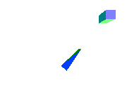
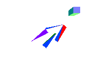
track object (requires bone; 15–30 points)

After applying other transformations (including positioning and rotation), rotate the object to the bone’s tip points toward the named object. This should be a minimal rotation to achieve that goal, staying as close to the previous orientation as possible.

Basic (15 points)

Rotation and negative length (5 points)

Tracking parent and target (10 points)

trackroll primary axis secondary (requires track; 10–20 points)

After applying other transformations (including positioning and rotation), rotate the object to the bone’s tip points toward the named primary object. There are many such rotations; pick the one that points the bone’s axis points toward the named secondary object as much as possible. Axis will always be one of +x, -x, +y, or -y.

Basic (10 points)

Tracking parent and target (10 points)

trackscale object (requires track; 10 points)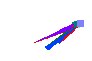

Like track, but also scale along the object’s z axis to that the tip of the bone exactly reaches the given object. Do not scale along the object’s other two axes.

trackstretch object (requires trackscale; 5 points)

Like trackscale, but also scale uniformly along the object’s x and y axes such that the volume of the bone is conserved.

fabrik object iterations (20–35 points)

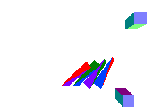
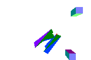
Use FABRIK to perform inverse kinematics, where the IK chain consists of this bone and all its bone parents.

Recall that one iteration of FABRIK moves the bone tip to object, then moves the chain root back to its starting location. Compute iterations iterations in total.

Each frame should begin the iteration from the positions provided by any position and quaternion commands. None of the bones in an IK chain will have a track or related command.

FABRIK produces the origins and tips of a chain of bones. Use the same math as position and track to align the bones with these points.

Basic (20 points)

With moving root (15 points)

1.2 make fluid file=filename (70–120 points)

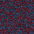
This is not an extension of any other assignment. You’ll output 2D fluids directly to the pixels of an image file (I guess we could say it’s an extension of HW0?).

Use back-advection to provide unconditionally stable simulations. When back-advecting off the grid, assume velocity is 0 and temperature is equal to the nearest on-grid temperature.

pngs width height filename frames

same syntax and semantics as HW0.

Each pixel in the image will represent a cell in a Eulerian fluid grid. Bigger images = higher-resolution fluids. Every cell will be full of fluid.

heat h bouyancy mag (70 points)

To create motion in the fluid, track something we’ll call the temperature of each pixel. We won’t simulate temperature-based expansion, but will approximate temperature-based buoyancy.

We’ll let temperature range from -1 to 1. Each pixel experiences an upward force with strength temperature × bouyancy pixels / frame².

The input h represents a rate of heat transfer into the fluid. The bottom row of pixels is heated, so t' = h + (1-h)t each frame; the top row is cooled, so t' = -h + (1-h)t each frame.

Use heat as the color of each pixel. Linearly interpolate between the following colors:

Temperature	Color
1	#ff0000
0	#000000
-1	#00B2FF

If temperatures are outside this range, you may color them in an implementation-defined manner.

For the first frame, set each cell to have a random temperature between −mag and +mag. This randomization breaks symmetry and gets the simulation started. Because of randomization, each run of a given file will produce a different result (but with the same overall dynamics).

diffuse rate (10 points)

Diffuse heat at the given rate each frame using a discrete Gaussian filter with rate as t.

viscosity rate (10 points)

Diffuse velocity at the given rate each frame using a discrete Gaussian filter with rate as t.

subsample n (10 points)

Render one image every n frames, where n is a positive integer.

for example, if the frames in the pngs is 100 and the n in subsample is 4 then you’ll simulate 400 frames but render only 100 images.

confine (requires viscosity; 10 points)

The linear weights involved in advection and the linear approximation of incomprehensibility created by using a matrix both tend to add unwanted numerical viscosity.

As a work-around, if the word confine appears in the input file then measure the kinetic energy of the fluid before each of these steps and artificially scale all velocities afterward to restore the previously-measured kinetic energy.

tconfine (requires diffuse; 10 points)

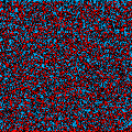The linear weights involved in advection tends to add unwanted numerical diffusion.

As a work-around, if the word tconfine appears in the input file then measure mean and variance of the temperatures fluid before each advection step and artificially shift and scale all temperatures afterward to restore the previously-measured mean and variance.

Other examples

Combined viscosity and diffusion:

Intense starting temperatures with no heating:

Combined confinement:

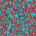
A 40s 720p simulation input file and result (in video player)

1.3 make springs file=filename (50–120 points)

This is not an extension of any other assignment. Rather, it outputs input files for HW3.

This is a mass-spring simulation with moving spheres, fixed planes, and springs. We discussed several approaches to this in class. To replicate my results, each iteration

1. draw a frame
2. move balls based on gravity and accumulated spring forces
3. move anchors
4. accumulate spring forces on each ball (without moving them)
5. resolve ball-ball collisions from first ball in file to last, moving them to not overlap and updating their velocity
6. resolve ball-anchor collisions, moving them to not overlap and updating their velocity
7. resolve ball-wall collisions, moving them to not overlap and updating their velocity

I did this in a single pass per time step, acting on the balls in the order I created them. Ball-ball collisions are resolved in order of the first ball in the pair, so the collision of the first and last ball is resolved before the collision of the second and third ball.

This order does mean that a later action cases an earlier fix to be partially undone, but I wanted something easy to describe to increase the chances everyone’s code would make the same animation. That said, I’m not looking for exact similarity: rather, I’m looking for the overall right kind of dynamics.

txts w h base frames

Create frames different input files for HW3. Each should begin with png w h base-frame.png where frame is a 3-digit zero-padded number between 0 and frames − 1. Each should be named base-frame.txt.

If the input file opens with

txts 30 40 example- 12

when it should make 12 new text files, named example-000.txt through example-011.txt. The last of these would start with the line

png 30 40 example-011.png

pass through

Any line that is not a command you’ve implemented for this assignment should be passed through as-is in every generated file.

If the input file contains

txts 30 40 example- 1

sphere 1 -0.8 -1 0.5
sphere 0 0 -1 0.3

sun 1 1 1

then, because the only line that starts with a HW5 keyword is txts, the output file will be

png 30 40 example-000.png

sphere 1 -0.8 -1 0.5
sphere 0 0 -1 0.3

sun 1 1 1

wall A B C D

Create a barrier ensuring that all balls will remain entirely in the region of space where Ax+By+Cz+D \ge 0.

This line is used only internally and does not appear in any form in the resulting output files.

This barrier is invisible. HW3’s visible variant was plane A B C D, but visible planes and interacting walls should be handled separately.

ball p_x p_y p_z   v_x v_y v_z

Create an animated ball at location (p_x, p_y, p_z) with velocity (v_x, v_y, v_z). Use the currently active radius and mass for the ball.

Each ball line in the input file becomes a sphere line in the output file; in particular, sphere c_x, c_y, c_z, r where (c_x,c_y,c_z) is the sphere’s center location on that frame and r is the spheres radius.

ball property specification (extra 5 if do both mass and elasticity)

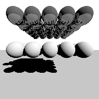Each of the following sets a value that will be applied to balls created after it. Each may be overridden by appearing multiple times in the input. Each is used only internally and does not appear in any form in the resulting output files.

radius r

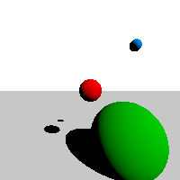The radius of subsequent balls. At least one radius command will always precede the first ball command.

mass m (5 points)

The mass of subsequent balls. If no mass has been encountered, use mass 1.

elasticity k (10 points)

The elasticity of subsequent balls. If no elasticity has been encountered, use elasticity 1.

In a ball-wall or ball-anchor collision, the coefficient of restitution used should be the ball’s elasticity. In a ball-ball collision, use the mean of the two elasticities.

gravity x y z (requires ball, radius, wall, and txt; 30 pts)

Accelerate all balls by \vec g = (x,y,z) / frame².

Recall that motion under acceleration works as follows:

• new \vec v = old \vec v + \Delta t \vec g
• new \vec p = old \vec p + \Delta t old \vec v + \frac{1}{2}\Delta t^2 \vec g

anchor p_x p_y p_z   v_x v_y v_z (15 pts)

Like ball, except an anchor ignores physics; instead it moves at a constant velocity, passing through walls and other anchors. Balls hitting anchors should act like they hit a wall (i.e., use only their own elasticity, not that of the anchor) but should correctly handle velocity added by hitting a moving anchor.

subsample n (10 pts)

For each frame, perform n distinct updates. For example, if n=10 then instead of one update of 1 time unit per frame you’d do 10 updates of 0.1 time unit each per frame.

The math should be such that this makes spring and collision computations more precise but does not change the result of freely-moving balls at all.

springconst k (requires subsample, mass, and elasticity)

The spring constant of subsequent springs. If no springconst has been encountered, use springconst 0 – i.e., ignore the springs.

For stability of simulation, it is recommended that input files keep \dfrac{\text{springconst}}{\text{subsample}} < 1.

tri n   a_x a_y a_z   b_x b_y b_z   c_x c_y c_z (requires springconst and anchor; 35 pts)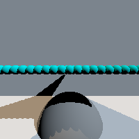

Create a triangle of balls by interpolating between the three given corner ball positions with n+1 balls per side of the triangle. Attach springs in a triangular grid.

Set all balls to initial velocity 0 and all springs to rest length = their initial length.

tri 3 … would produce 10 balls 18 springs arranged as illustrated in the following ASCII art:

      c
     / \
    * - * 
   / \ / \
  * - * - * 
 / \ / \ / \
a - * - * - b

tet n   a_x a_y a_z   b_x b_y b_z   c_x c_y c_z   d_x d_y d_z (requires tri; 10 pts)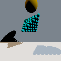

Create a tetrahedreon of balls by interpolating between the four given corner ball positions with n+1 balls per edge of the tetrahedron. Attach springs in a tetrahedral grid.

Set all balls to initial velocity 0 and all springs to rest length = their initial length.