1 Overview

This assignment will have you render animations as a series of images, using the pngs command from HW0.

If you didn’t figure out how to display animations during HW0, you should definitely do that now.

Most animator-specified computer animations are the combination of two components: a scene graph and time-varying parameters.

1.1 Scene Graph

In this assignment we’ll replicate a version of the scene graph used in many animation tools.

Each object will have

• a parent, which is either another object or the world
• an origin, which is a 3-vector defaulting to (0,0,0) (not in the required part of the assignment)
• a scale, which is a 3-vector defaulting to (1,1,1) (not in the required part of the assignment)
• a position, which is a 3-vector defaulting to (0,0,0)
• an orientation, which will be given either in Euler or Quaternion form defaulting to \langle 1;0,0,0 \rangle
• geometry, given as vertices and triangles similar to HW2

A matrix to position the vertices of an object can be created by multiplying several component matrices together: [\cdots] \quad T_O \; T_P \; R \; S \; T_O^{-1} where T_O is a translation matrix moving (0,0,0) to the object’s origin; T_P is a translation matrix moving (0,0,0) to the object’s position; S is a scaling matrix, the diagonal of the object’s scale; R is a rotation matrix defined by the object’s orientation; and [\cdots] is the matrix for the object’s parent, or nothing if the parent is the world.

Matrices are not necessary in this case: you can also apply the operations directly as q \odot ((p - O) \otimes S) \odot q^{*} + P + O where \otimes is element-wise multiplication, q is the normalized orientation quaternion, q^{*} is the conjugate of q, and \odot is the quaternion multiplication operator. If there are more than a few points, though, constructing the matrix first is more efficient.

The camera is a special object with no geometry. To position an object’s points for rendering by the camera, use C^{-1}\, O where C is the matrix (constructed as described above) for the camera and O is the matrix (constructed as described above) for the object. Recall that:

• For any two matrices A and B, (AB)^{-1} = B^{-1} A^{-1}
• The inverse of a translation by (x,y,z) is a translation by (-x,-y,-z)
• The inverse of a scaling by (x,y,z) is a translation by (1/x, 1/y, 1/z)
• The inverse of a rotation matrix R is the transpose of that matrix R^{-1} = R^{T}
• The inverse of a rotation quaterion q is its conjugate q^{*}

You can compute the inverse of a transformation matrix more accurately using the above rules than you can using a generic matrix inversion routine.

 

All this organization may seem like more bother than its worth, but scene graphs make complicated and interesting animation much easier to create.

1.2 Time-varying parameters

We’ll add animation by allowing various numbers, such as the coordinates of an object’s position vector, to be defined by a time-varying variable.

Every file will have access to two variables: f, which is equal to the current frame number, and l, which is the number of frames in the animation.

You’ll implement several ways of defining additional variables. To avoid the complexities of a full programming language, we’ll guarantee that regardless of which variable definition forms you define

• each variable will be defined only once; no x = x + 1-type reassignments;
• each variable will be defined before it is used; and
• variable definitions will be individually simple to parse: no parentheses or the like.

The above limitations will make writing the input files a bit tedious, but will keep parsing them straightforward.

Some full animation systems will animate vectors separately from their coordinates, for example using slurps (spherical linear interpolation) or hlerps (hyperbolic linear interpolation). Those can be decomposed into per-coordinate trigonometry and other more involved functions; to keep the input files from getting out of hand we’ll only deal with them in that form.

1.3 Code organization

Start with a copy of (at least the required parts of) your HW2 code.

HW2’s trif and related commands indexed a single global list of points. For HW4 the indices will reset each time an object command is given; thus trif 1 2 -1 is a triangle connecting the first two points of the most recent object with the last point provided.

You won’t need loadm directly; the modelview matrix will be given by the object transformations isntead. We will use loadp exactly as HW2 did.

You will almost certainly need two maps: one mapping variable names to their definitions and one mapping object names to their corresponding objects.

The file will be organized so that what you store can be quite simple if you are willing to re-read the file once per frame. Because variables are defined before use, re-reading will allow you to store just the variable values at that frame rather than full defining expressions. Because each object’s position, orientation, scale, and parent are defined before its geometry and because parent objects are defined before child objects, it is possible implement the required functionalty storing only the transformation matrix for each object, rendering the geometry immediately instead of storing it.

That said, using more involved data structures and code organization may make your code easier to reason about and may be necessary to implement some of the optional components.

2 Required Features

The required part is worth 50%

I use two words for information you should ignore during rendering: fps for the frame per second used in my reference animated PNGs and # for comments. Because you’ve been ignoring unknown keywords since HW0, the fact these are in the files shouldn’t cause you any problems.

2.1 Drawing objects

pngs width height filename frames

same syntax and semantics as HW0.

loadp a_{1,1} a_{1,2} a_{1,3} a_{1,4} a_{2,1} a_{2,2} … a_{4,4}

As in HW2. Will appear only once, before any objects

color r g b

As in HW2.

object name parent

Begin a new object with the given name. The name may be used to indicate this object as the parent of later objects. The special name world may appear in the parent field to indicate the object has no parent.

You may assume that the name is unique in the file, an ASCII identifier (i.e. no spaces or fancy characters), and not world; and that parent is either world or the name of an object that appeared previously in this file.

Every object line will be followed by its transformations (if any) and then its geometry.

position x y z

An optional transformation of the object; if missing, defaults of position 0 0 0.

Describes the position of this object relative to its parent, in a coordinate system modified by its parent’s position, orientation, and scale but not modified by this object’s orientation or scale.

Each object will have at most one position. If present, it will precede any geometry for that object.

quaternion w x y z

An optional orientation transformation of the object; if missing and no other orientation command is provided, defaults to quaternion 1 0 0 0.

Describes the orientation of this object relative to its parent, in a coordinate system modified by its parent’s position, orientation, and scale but not modified by this object’s position or scale.

Each object will have at most one orientation, which may be quaternion or one of the alternatives given in the optional features section. If present, it will precede any geometry for that object.

xyz x y z

As in HW2. Will only appear after an object and its transformations. Note that point indexing resets with each new object.

trif i_1 i_2 i_3

As in HW2. Will only appear after an object and its transformations. Note that point indexing resets with each new object.

2.2 Basic animation

add dest a b

Create a new variable called dest that is equal to a + b

sub dest a b

Create a new variable called dest that is equal to a - b

mul dest a b

Create a new variable called dest that is equal to a \times b

div dest a b

Create a new variable called dest that is equal to a \div b

pow dest a b

Create a new variable called dest that is equal to a^b

sin dest a

Create a new variable called dest that is equal to \sin(a), where a is specified in degrees.

cos dest a

Create a new variable called dest that is equal to \cos(a), where a is specified in degrees.

Animate transforms

Allow the arguments of position and quaternion, as well as the mathematics operators above, to be any mix of variables and numbers.

---

3 Optional Features

3.1 More Transformations (5–35 pt)

origin o_x o_y o_z (5 pt)

An optional origin of the object; if missing defaults to origin 0 0 0.

Describes the origin around which other transforms occur.

Each object will have at most one origin; if present, it will precede any geometry for that object.

scale s_x s_y s_z (10 pt)

An optional transformation of the object; if missing defaults to scale 1 1 1.

Describes the axis-aligned components of the scale of this object relative to its parent, in a coordinate system modified by its parent’s position, orientation, and scale but not modified by this object’s position or orientation.

Each object will have at most one scale; if present, it will precede any geometry for that object.

anyscale s_x s_y s_z w x y z (10 pt)

An optional transformation of the object.

Describes the scale of this object along arbitrary axes as given by a quaternion. The axes of the scale should be rotated by the given quaternion, but the object itself should not. The simplest way to achieve that is to rotate by the inverse of the quaternion, scale along the principle axes by the given factors, and then rotating back.

Each object will have one scale or one anyscale or neither; if either is present, it will precede any geometry for that object.

euler xyz r_1 r_2 r_3 (10 pt)

An alternative representation of the orientation of an object.

Describes orientation as three consecutive principle-axis rotations. The order of the rotations will be given by the xyz argument, which will contain three letters (x, y, and z) in an arbitrary order (e.g. yxz or zxy or …). First rotate the object r_1 degrees around the axis given by the first letter, then r_2 degrees around the axis given by the second letter, then r_3 degrees around the axis given by the third letter. Note that first means as the left-most matrix, so euler xyz is the product of three matrices R_z R_y R_x.

3.2 More things animated (5–30 pt)

Animate vertices (5 pt)

Allow the coordinates of vertices to be variables or values. This may mean that the vertices of a triangle are sometimes all the same location in space.

Animate colors (10 pt)

Allow the coordinates of colors to be variables or values. Variables may go outside the 0–1 range and if so should be clamped to the nearest legal value before display,

iflt x y (15 pt)
else
fi

If x < y, perform the commands between iflt and the next else but not between the else and the next fi. Otherwise, perform the commands between else and fi, not between iflt and else.

These commands may wrap arbitrary content, including geometry, variable definitions, objects, transforms, etc. To simplify parsing, one iflt will never contain a nested iflt.

3.3 Animations used in keyframes (10–45 pt)

piecewise dest v_1 t_1 v_2 t_2 … t_n v_{n+1} (10 pt)

Create a new variable called dest out of a set of old variables using the logic

if f \le t_1: use v_1
else if f \le t_2: use v_2
…
else if f \le t_n: use v_n
else use v_{n+1}

lerp dest t_1 v_1 t_2 v_2 … t_n v_n (10 pt)

Define a variable dest to be the a piecewise-linear interpolation of several values. Arguments are (frame, value) pairs (with fractional frames permitted) and are given in increasing order of t (i.e., t_i < t_{i+1}). Prior to t_1, dest is v_1. After t_n, dest is v_n. Between t_i and t_{i+1}, dest changes linearly from v_i to v_{i+1}.

bez dest t_1 a_1 b_1 c_1 t_2 a_2 b_2 c_2 … c_{n-1} t_n a_{n} (15 pt)

Similar to lerp, but using explicit cubic Bézier curves¹ instead of linear interpolation between t values.

The control points between t_i and t_{i+1} are a_i, b_i, c_i, and a_{i+1}.

Some variant of this function is used by most keyframe animation systems and can be edited directly in the expert mode or graph editor or the like.

You might find our Bézier reference useful

autobez dest t_1 v_1 t_2 v_2 … (10 pt)

A shorthand way of defining bez, some variant of which is commonly used in keyframe animation systems as the initial guess at desired tweening.

The input format matches lerp: a set of (frame, value) pairs. Control points are determined by computing slopes at each keyframe: the slope at t_i is \displaystyle\frac{v_{i+1}-v_{i-1}}{t_{i+1}-t_{i-1}} and the control points on either side of v_i are computed by extending that slope out ⅓ of the way to the next keyframe.

For the first and last keyframe, compute the slope with the keyframe and its one neighbor instead of its two neighbors.

The command autobez x5 3 -2.0 9 7.0 27 1.0 computes slopes \frac{7-(-2)}{9-3} = \frac{3}{2}, \frac{1-(-2)}{27-3} = \frac{1}{8}, and \frac{1-7}{27-9} = \frac{-1}{3} and thus sets x5 to

• -2.0 for frames 0 through 3
• The Bézier with control points -2.0, 1.0, 6.75, 7.0 between frames 3 and 9
• The Bézier with control points 7.0, 7.75, 3.0, 1.0 between frames 9 and 27
• 1.0 for frames 27+

3.4 Camera support (0–30 pt)

camera parent (20 pt)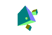

A file may contain a single camera command, which is followed by the camera’s parent. The input treats the camera like an object (with position, quaternion, etc), except it may not have geometry. See the overview for guidance on how to draw with a moving camera.

For this set of optional points, you only need to support the specific parent value world.

Camera in scene graph (10 pt)

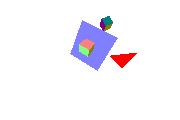Let the camera have a parent that is an object, not just the world. Let other objects use camera as their parent.

---

1. Explicit Bézier curves are also called nonparametric Bézier curves or polynomials in the Bernstein basis. They can equivalently treated as either Bézier curves with scalar instead of vector control points or 2D Bézier curves where the t axis control points are evenly spaced.↩︎